\newpage

Pset4

Name: Divy Chandra

Cohort: SC06

Student ID: 1005246

---

Problem 1

Two types of solar cells are:

1. Monocrystalline

   Advantage: They are the most efficient solar panels, with an efficiency of about (15% - 20%)

   Disadvantage: They are quite expensive

2. Polycrystalline

   Advantage: They are cheaper and easier to produce than monocrystalline solar panels

   Disadvantage: Their efficiency is lower than that of monocrystalline cells (13% - 16%)

Problem 2

It is known that \(I_o\) (the reverse saturation current) is directly proportional to the intensity of light incident on the solar panel.

Also note that:

\(I_{sc} = I_o(e^{\cfrac{eV}{k_B T}} - 1)\)

\(V_{oc} = \cfrac{K_B T}{e} ln\left(\cfrac{I_{sc}}{I_o} + 1\right)\)

From the first formula, we note that \(I_{sc}\) is proportional to the \(I_o\) which implies that it is also proportional to the intensity of light incident on the solar panel.

Hence, when the light intensity is doubled, we get the new \(I_{sc} = 300 mA\)

Using the first formula in the second formula, we can write:

\(I_{sc} = I_o(e^{\cfrac{qV}{k_B T}} - 1)\)

\(\cfrac{I_{sc}}{I_o} = e^{\cfrac{qV}{k_B T}} - 1\)

For \(500 W/m^2\), we have:

\(\cfrac{0.15}{I_o} = e^{\cfrac{e 0.53}{k_B T}} - 1\)

For \(1000 W/m^2\), we have:

\(\cfrac{0.3}{I_o} = e^{\cfrac{qV_{oc}}{k_B T}} - 1\)

Dividing the two equations:

\(\cfrac{1}{2} = \cfrac{e^{\cfrac{q 0.53}{k_B T}} - 1}{e^{\cfrac{qV_{oc}}{k_B T}} - 1}\)

\(e^{\cfrac{qV_{oc}}{k_B T}} - 1 = 2 \times e^{\cfrac{q 0.53}{k_B T}} - 2\)

\(e^{\cfrac{qV_{oc}}{k_B T}} = 2 \times e^{\cfrac{q 0.53}{k_B T}} - 1\)

Log on both sides:

\(\cfrac{qV_{oc}}{k_B T} = ln\left( 2 \times e^{\cfrac{q 0.53}{k_B T}} - 1 \right)\)

we know that \(q = 1.6 \times 10^{-19} C\) and \(K_B T = 4.149 \times 10^{-21} J\). Using these values, we calculate and simplify the above expression to:

\(38.56 V_{oc} = 21.13\)

\(\color{blue} V_{oc} = 0.548 V\)

\(\color{blue} I_{sc} = 300 mA\)

\newpage

Problem 3

i)

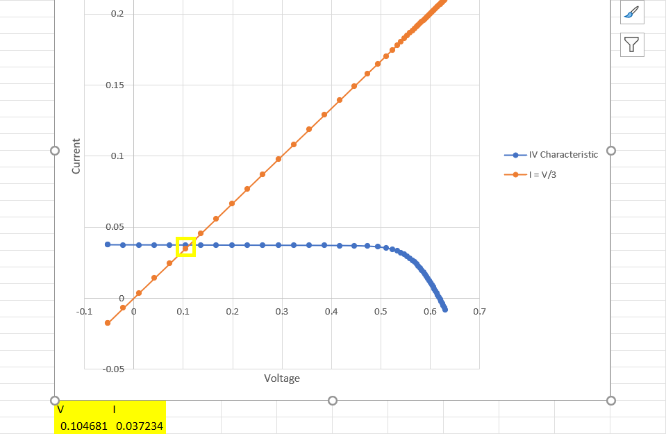
From the graph above,

\(\color{blue} V = 0.104681 V\) \(\color{blue} I = 0.037234 A\)

ii)

\(P = 0.104681 \times 0.037234 W\)

\(\color{blue} P = 0.0039 W\)

iii)

\(\% Conversion = \cfrac{P_{delivered}}{P_{incident}} \times 100\% = \cfrac{0.0039}{1000 \times 10^{-4}} \times 100\%\)

\(\color{blue} \% Conversion = 3.9 \%\)

\newpage

iv)

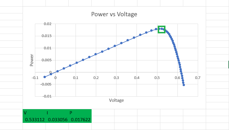
From the graph above,

\(\color{blue} P_{max} = 0.0176 W\)

v)

\(V_{oc} = 0.62 V\)

\(I_{sc} = 0.037 A\)

\(FF = \cfrac{P_{max}}{V_{oc} I_{sc}} = \cfrac{0.0176}{0.62 \times 0.037}\)

\(\color{blue} FF = 0.767\)

vi)

\(\eta = \cfrac{P_{max}}{P_{in}} = {0.0176}{0.1}\)

\(\color{blue} \eta = 0.176\)